Basic data processing tutorial

1. Package installation

install.packages("chron",repos = "http://cran.us.r-project.org")
install.packages("readxl", repos = "http://cran.us.r-project.org")
install.packages("ggplot2",repos = "http://cran.us.r-project.org")

Be aware that some packages don’t work with some versions of R. For example “tidyr” only works with new versions of R. If you have more than one version of R (not R Studio) installed in the pc R Studio gives you the option of choosing which version you want to use: tools->global options-> R version. Additonally, when working on the university computers sometimes you might need to install the packages in other than the default library (H drive) due to permission restrictions. Use the command .libPaths(your path) to change the default library location. After installing the packages don’t forget to load them.

library(chron)
library(readxl)
library(ggplot2)

Set your working directory. If you are working with multiple files from different folders or you want to save the outputs in different folders, you can always create a vector with your folder path.

setwd("C:\\Users\\r01ac17\\Desktop\\tutorial\\") # R will search for files in this folder
save.folder<-"C:\\Users\\r01ac17\\Desktop\\tutorial\\plots\\"
dir.create(save.folder) # create directory

#2. Import data We will work with elasmobranchii data from the Scottish West Coast Survey for commercial fish species dowloaded from http://www.iobis.org/mapper/. Use the command below to download the data.txt from the Github into your directory. For the excel data, download it directly from GitHub and place it in your working directory. ```{r error=TRUE} download.file(“https://raw.githubusercontent.com/Anofia/Basic-R-tutorial/master/data.txt”, destfile = “data.txt”)

data<-read.table(“data.txt”) data<-read.table(“data.txt”, fill=TRUE) #fill=TRUE will solve the error by filling the gaps with NA data<-read.table(“data.txt”, fill=TRUE, sep=”,”) #data is all in one column; wrong sep data<-read.table(“data.txt”, fill=TRUE, sep=”\t”) #but colnames are not defined data<-read.table(“data.txt”, fill=TRUE, sep=”\t”, header=TRUE) head(data)

To import data form excel you can use the folling code:
```{r}
data.excel<-read_excel("data.xlsx", sheet=1) # if you have multiple sheets you can choose which one to load

##3. Data manipulation Lets see if there are changes in the number of individuals per season and year. First we create separate columns with years and months.

dates<-as.Date(data$datecollected)
head(dates) # what is wrong with this???
head(data$datecollected) # dates are in format dd/mm/yyyy
dates<-as.Date(data$datecollected, format="%d/%m/%Y")
head(dates) #perfect!
data$month<-format(dates,"%m")
data$year<-format(dates,"%Y")

Because each row is an individual, we create a new column with a sequence of 1 to sum the number of indivuals per species, year and month

data$n<-1
n.ind<-aggregate(n ~ tname + month+ year, data=data, FUN = sum)
colnames(n.ind)
colnames(n.ind)<-c("species","month","year","n") #change colnames
colnames(n.ind)

length(unique(n.ind$species)) #check how many species we have

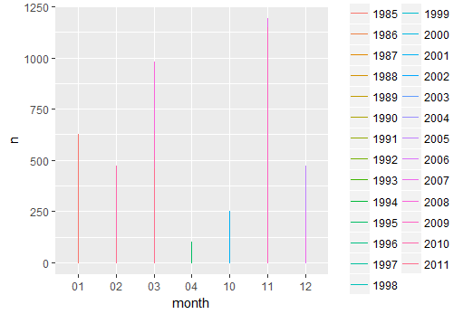
Using ggplot2 (see tutorial for ggplot2 as well) we will plot the number of individuals per month and per year for all the species combined and for each individual species.

ggplot(data=n.ind,aes(x=month, y=n, colour=year)) + geom_line() # this doesn't look good, why?
class(n.ind$month)

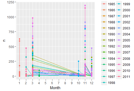
ggplot(data=n.ind,aes(x=as.numeric(month), y=n, colour=year)) + geom_line() + geom_point() +scale_x_continuous(breaks=seq(1,12,1)) +xlab("Month")

ggplot(data=n.ind,aes(x=as.numeric(month), y=n, colour=year)) + geom_line() + geom_point() + facet_wrap(~species,scales=("free_y")) +scale_x_continuous(breaks=seq(1,12,1)) +xlab("Month")

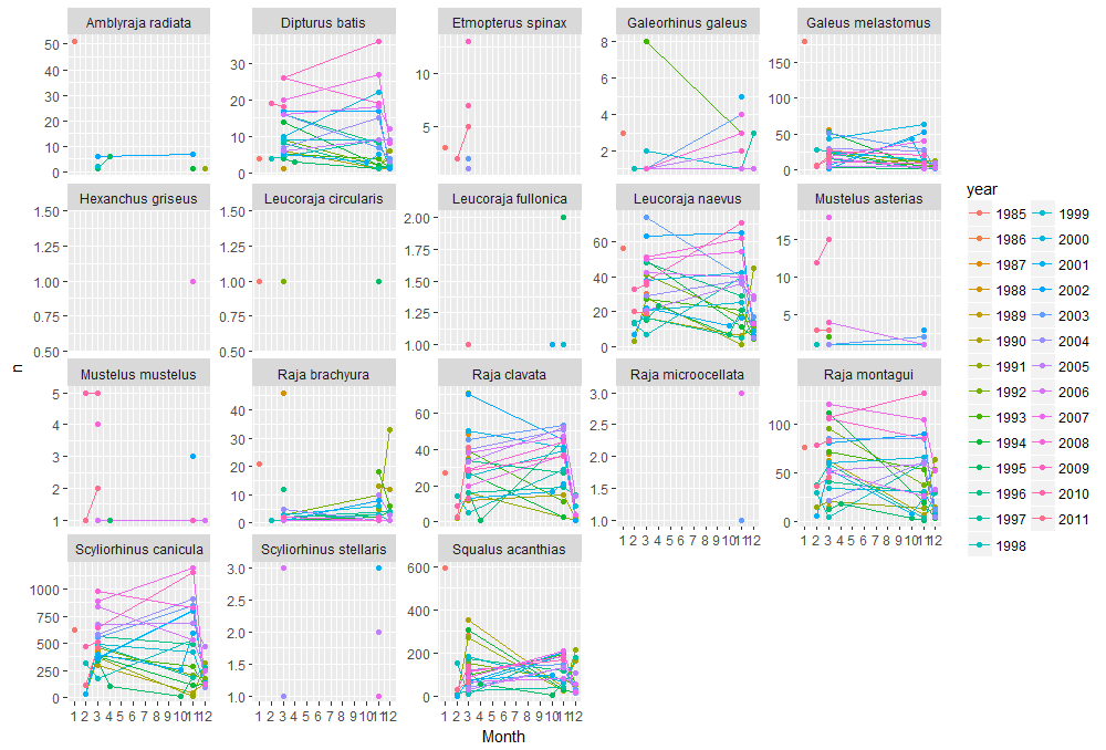
For many species we only have a few observations. So lets look at only at one of the species that have higher values.

unique(n.ind$species)
sp<-"Squalus acanthias" #variable with the species name that you want to select
sp.data<-data[which(data$tname==sp),] #select only rows for the selected species
head(sp.data)

#try to change sp to "Scyliorhinus canicula" and re-run the sp.data
sp<-"Scyliorhinus canicula" #variable with the species name that you want to select
sp.data<-data[which(data$tname==sp),] #select only rows for the selected species
head(sp.data)

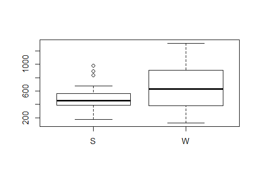
As we have winter and spring data for Scyliorhinus canicula, lets check if there are any differences between seasons. First we create a new column with S for spring and W for winter using the function ifelse. Second we aggregate the total number of individuals per season and year. We can use a boxplot to see the differences between spring and winter and a t.test to see if this differences are significant.

sp.data$season<-ifelse(as.numeric(sp.data$month)%in% c(3,4), "S", "W")
colnames(sp.data)
n.sp<-aggregate(n ~ season + year, data=sp.data, FUN = sum)
boxplot(n~season, n.sp)
t.test(n~season, n.sp)

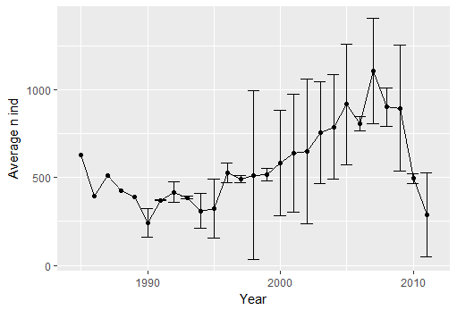
Now lets see if there are differences between the year for the overall average and for each season separately.

mean.year<-aggregate(n ~ year , data=n.sp, FUN = mean) #mean
sd.year<-aggregate(n ~ year , data=n.sp, FUN = sd)#sd
year<-merge(mean.year, sd.year) #what is wrong?
year<-merge(mean.year, sd.year, by="year") # many functions will not give an error but they are not doing it properly - always check your data along the way

colnames(year)
colnames(year)<-c("year","mean","sd") #change colnames
colnames(year)

ggplot(year, aes(x=as.numeric(year),y=mean))+geom_line()+geom_point()+xlab("Year")+ylab("Average n ind") + geom_errorbar(year, mapping=aes(x=as.numeric(year), ymin=mean-sd, ymax=mean+sd))

#plot n ind per year for each season
ggplot(n.sp, aes(x=as.numeric(year),y=n, color=season))+geom_line()+geom_point()+xlab("Year")+ylab("N ind")

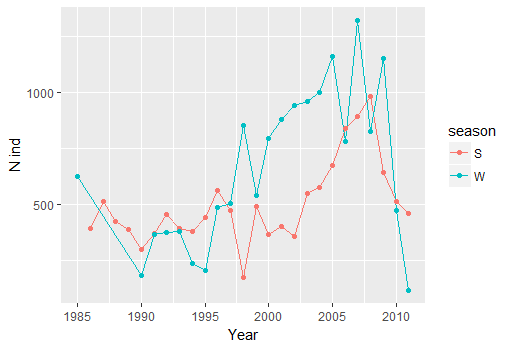
You can see that from 1997 there is an inversion in the general trend, with more sharks in winter than spring - lets see if there is any relation with environmental variables. To start we calculate the both the mean and max temperature per season and year. Notice that the data has a lot of NA. Arithmetic functions on NA yield NA. Aggregate automatically removes NA. But you can also remove the rows with NA in it yourself. ```{r error=TRUE} colnames(sp.data) #mean sst mean(sp.data$temperature) #NA mean(sp.data$temperature, na.rm=TRUE)

head(is.na(sp.data$temperature)) # this tells you which data are NA na.sp.data<-sp.data[!is.na(sp.data$temperature), ] #! means the contrary: you want the observations that are not NA

mean.sst<-aggregate(temperature ~ season + year, data=sp.data, FUN = mean) #aggregate automatically deals with NAs colnames(mean.sst)<-c(“season”,”year”,”mean.temp”) max.sst<-aggregate(temperature ~ season + year, data=sp.data, FUN = max) colnames(max.sst)<-c(“season”,”year”,”max.temp”) #lets add temperature to n.sum n.sp<-merge(n.sp,mean.sst,max.sst, by=c(“season”,”year”)) # merge only allows to merge 2 data frames n.sp<-cbind(n.sp, mean.sst$mean.temp, max.sst$max.temp) colnames(n.sp)<-c(“season”,”year”,”n”, “mean.temp”,”max.temp”)

We can use a simple correlation test to see if there is any significant relation between temperature (max or mean) and number of individuals. Ploting the data with trend lines will allow you to see what is going on.
```{r error=TRUE}
cor.test(n.sp$n, n.sp$mean.temp) # there is no correlation between n ind and mean temperature
cor.test(n.sp$n, n.sp$max.temp) # there is no correlation between n ind and max temperature

plot(n~mean.temp, n.sp, main="Mean sst")
# Add fit lines
abline(lm(n~mean.temp, n.sp), col="red") # regression line (y~x)
lines(lowess(mean.temp,n), col="blue") # lowess line (x,y) - error: R doesn't know where to get n or mean.temp
lines(lowess(n.sp$mean.temp,n.sp$n), col="blue") # lowess line (x,y)

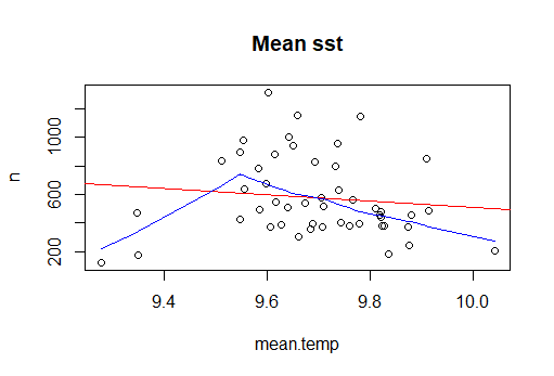
It seems that there are some extreme values in the data: this can bias/change the fit estimates and predictions. In some cases outliers don’t have to be removed, it depends if the data makes sense or if it as sampling error. other ways to deal with outliers are data transformation or use a different model. Two very good book on the subject are “Analysing ecological data” and “A beginner’s guide to R” for Alain Zuur. For this tutorial, we will treat extreme values as outliers to see the difference between the predictions. There are several methods to detect extreme values. we will use Cooks Distance method. ```{r error=TRUE} mod<- lm(n~mean.temp, data=n.sp) cooksd <- cooks.distance(mod) #Cooks Distance method plot(cooksd, pch=””, cex=2, main=”Influential Obs by Cooks distance”) # plot cook’s distance abline(h = 4mean(cooksd, na.rm=T), col=”red”) # add cutoff line; In general use, those observations that have a cook’s distance greater than 4 times the mean may be classified as influential. This is not a hard boundary. text(x=1:length(cooksd)+1, y=cooksd, labels=ifelse(cooksd>4mean(cooksd, na.rm=T),names(cooksd),””), col=”red”) # add labels outliers<-which(cooksd>4mean(cooksd, na.rm=T))

#lets remove outliers and re check the correlations/plots n.sp.out<-n.sp[-outliers,] plot(n~mean.temp, n.sp.out, main=”Mean sst”)

Add fit lines

abline(lm(n~mean.temp, n.sp.out), col=”red”) # regression line (y~x) lines(lowess(n.sp.out$mean.temp,n.sp.out$n), col=”blue”) # lowess line (x,y) cor.test(n.sp.out$n, n.sp.out$mean.temp) # now the correlation between mean temperature and n indivuals is significative.

<center><img src="../Plot8.png" alt="Img" style="width: 800px;"/></center>

<center><img src="../Plot9.png" alt="Img" style="width: 800px;"/></center>

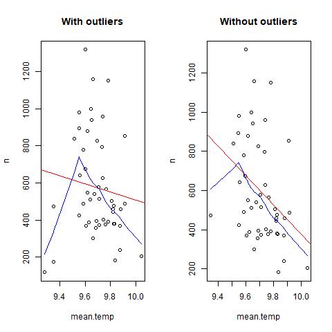
One last thing before finish, lets plot the data with and without outliers side by side in and save it as jpeg.
```{r error=TRUE}
jpeg(filename=paste0(save.folder,"outliers.jpg")) # this opens the image
par(mfrow=c(1,2))
plot(n~mean.temp, n.sp, main="With outliers")
abline(lm(n~mean.temp, n.sp), col="red") # regression line (y~x)
lines(lowess(n.sp$mean.temp,n.sp$n), col="blue") # lowess line (x,y))

plot(n~mean.temp, n.sp.out, main="Without outliers")
abline(lm(n~mean.temp, n.sp.out), col="red") # regression line (y~x)
lines(lowess(n.sp.out$mean.temp,n.sp.out$n), col="blue") # lowess line (x,y))

dev.off () # this closes the image