Open Spatial Analysis 1 - Handling spatial data in R

During this tutorial you will learn how to deal with spatial data in R.

To follow the tutorial go to this link to download some of the data you will need. Once you’re there, click on the green Clone or download button.You can either clone the repository on your GitHub account (if you have one) or download as a zip file. Once you done, open an R or Rsudio session and set the working directory to the directory where you saved the repository.

The exercise is divided in three parts, followed by a summary and links to other useful resources:

1. Classes for Spatial Data in R and how to import the data

1.1. The `Spatial` class and its subclasses

1.2. Importing your data and making it spatial

1.3. Importing shapefiles

2. Visualising Spatial Data

2.1. Plotting lines, points and polygons

2.2. Projections and transformations

3. Geoprocessing

3.1. Buffer and intersect

3.2. Distance

4. Rasters

4.1. Import rasters and change projection

4.2. Some geoprocessing

5. Summary and useful links

1. Classes for Spatial Data in R and how to import the data

Data requires two types of information to be spatial:

coordinate values
a system of reference for these coordinates

The reason why we need the first piece of information is self-explanatory, we need an x and y location on the Earth where our features are located. The second piece of information is necessary because the Earth is shperical while a map is flat, so that when we want to represent spatial features on a 2-dimensional surface we need to translate from the spherical longitude/latitude system to a non-spherical coordinate system. Any other information attached to these locations, such as time, depth or height, is an attribute. There are different ways of representing spatial information, the main ones are:

points - a single location, such as a GPS reading of a species sighting
lines - a set of points connected by sraight line segments, such as a road
polygons - an area marked by one or more lines, such as a country
grids - a set of points or rectangular cells organised in a regular lattice

The first 3 are vector data models and we will look at them in the first three sections of this tutorial. The latter is a raster data model, representing continuous surfaces by using a regular tessellation. We will look at this type of data in the last part of this tutorial.

1.1. The `Spatial` class and its subclasses

All spatial objects in R belong to the class Spatial with just two slots:

a bounding box, a matrix of numerical coordinates with two columns (“min” and “max”) and two rows (x and y coordinates)
a CRS class object, a character string defining the coordinate system (proj4string).

The class Spatial has 10 subclasses. We can use the function getClass to see the definition of a class and its subclasses. If you don’t have the package sp already, install it with install.packages("sp").

> library(sp)

> getClass("Spatial")

Class "Spatial" [package "sp"]

Slots:
                              
Name:         bbox proj4string
Class:      matrix         CRS

Known Subclasses: 
Class "SpatialPoints", directly
Class "SpatialMultiPoints", directly
Class "SpatialGrid", directly
Class "SpatialLines", directly
Class "SpatialPolygons", directly
Class "SpatialPointsDataFrame", by class "SpatialPoints", distance 2
Class "SpatialPixels", by class "SpatialPoints", distance 2
Class "SpatialMultiPointsDataFrame", by class "SpatialMultiPoints", distance 2
Class "SpatialGridDataFrame", by class "SpatialGrid", distance 2
Class "SpatialLinesDataFrame", by class "SpatialLines", distance 2
Class "SpatialPixelsDataFrame", by class "SpatialPoints", distance 3
Class "SpatialPolygonsDataFrame", by class "SpatialPolygons", distance 2

All the subclasses extend the class Spatial, for example, the class SpatialPoints extends the class Spatial by adding a coords slot, which contains a matrix of point coordinates:

> getClass("SpatialPoints")
Class "SpatialPoints" [package "sp"]

Slots:
                                          
Name:       coords        bbox proj4string
Class:      matrix      matrix         CRS

Extends: "Spatial"

Known Subclasses: 
Class "SpatialPointsDataFrame", directly
Class "SpatialPixels", directly
Class "SpatialPixelsDataFrame", by class "SpatialPixels", distance 2

If any attribute is associated to the points then the classSpatialPoints is extended into SpatialPointsDataFrame by adding one more slots, the data.frame of the attributes.

> getClass("SpatialPointsDataFrame")
Class "SpatialPointsDataFrame" [package "sp"]

Slots:
                                                                  
Name:         data  coords.nrs      coords        bbox proj4string
Class:  data.frame     numeric      matrix      matrix         CRS

Extends: 
Class "SpatialPoints", directly
Class "Spatial", by class "SpatialPoints", distance 2

Known Subclasses: 
Class "SpatialPixelsDataFrame", directly, with explicit coerce

Use the function getClass to look at the other subclasses of Spatial and notice which slots they contain. What are the differences?

1.2. Importing your data and making it spatial

For this part of the tutorial we will use a dataset downloaded from GBIF containing occurrences of watervoles (Arvicola amphibius) in the UK. You will find the dataset voles.csv in the folder called data. It is a .csv file so we can use read.csv to read it into R:

> voles <- read.csv("./data/voles.csv", header = T, sep = "\t")
> str(voles)
'data.frame':	46570 obs. of  44 variables:
 $ gbifid                       : int  1586099341 1572202623 1572202621 1572202618 1572202617 1572202616 1572202615 1572202614 1572202613 1572202612 ...
 $ datasetkey                   : Factor w/ 78 levels "00c913d4-7148-46b3-9aa6-b2a158fa721b",..: 28 10 10 10 10 10 10 10 10 10 ...
 $ occurrenceid                 : Factor w/ 46568 levels "","0000a642-d4cc-4fbd-bb7d-5c35053c6e7b",..: 46568 22485 9720 40364 15379 17564 35261 43846 3354 43284 ...
 $ kingdom                      : Factor w/ 1 level "Animalia": 1 1 1 1 1 1 1 1 1 1 ...
 $ phylum                       : Factor w/ 1 level "Chordata": 1 1 1 1 1 1 1 1 1 1 ...
 $ class                        : Factor w/ 1 level "Mammalia": 1 1 1 1 1 1 1 1 1 1 ...
 $ order                        : Factor w/ 1 level "Rodentia": 1 1 1 1 1 1 1 1 1 1 ...
 $ family                       : Factor w/ 1 level "Cricetidae": 1 1 1 1 1 1 1 1 1 1 ...
 $ genus                        : Factor w/ 1 level "Arvicola": 1 1 1 1 1 1 1 1 1 1 ...
 $ species                      : Factor w/ 1 level "Arvicola amphibius": 1 1 1 1 1 1 1 1 1 1 ...
 $ infraspecificepithet         : logi  NA NA NA NA NA NA ...
 $ taxonrank                    : Factor w/ 1 level "SPECIES": 1 1 1 1 1 1 1 1 1 1 ...
 $ scientificname               : Factor w/ 2 levels "Arvicola amphibius (Linnaeus, 1758)",..: 1 1 1 1 1 1 1 1 1 1 ...
 $ countrycode                  : Factor w/ 1 level "GB": 1 1 1 1 1 1 1 1 1 1 ...
 $ locality                     : Factor w/ 3723 levels "","\"Haddiscoe, Wheatacre & Burgh Marshes\"",..: 1 1 1 1 1 1 1 1 1 1 ...
 $ publishingorgkey             : Factor w/ 49 levels "05c84e36-2006-4e3d-ad77-ebd529aa09c4",..: 11 17 17 17 17 17 17 17 17 17 ...
 $ decimallatitude              : num  51.5 53.3 53.2 53.3 53.1 ...
 $ decimallongitude             : num  0.22 -0.877 -1.179 -1.177 -1.18 ...
 ...

In order to make it spatial, we need to specify which columns contain the coordinates of the location of each occurrence and the coordinate reference system. The columns tha contain the spatial information we need are decimallatitude and decimallongitude, so we can use the function coordinates to set spatial coordinates to create a Spatial object:

> coordinates(voles) <- c("decimallongitude", "decimallatitude")    # eastings always go before northings in sp classes
> str(voles)
Formal class 'SpatialPointsDataFrame' [package "sp"] with 5 slots
  ..@ data       :'data.frame':	46570 obs. of  42 variables:
  .. ..$ gbifid                       : int [1:46570] 1586099341 1572202623 1572202621 1572202618 1572202617 1572202616 1572202615 1572202614 1572202613 1572202612 ...
  .. ..$ datasetkey                   : Factor w/ 78 levels "00c913d4-7148-46b3-9aa6-b2a158fa721b",..: 28 10 10 10 10 10 10 10 10 10 ...
  .. ..$ occurrenceid                 : Factor w/ 46568 levels "","0000a642-d4cc-4fbd-bb7d-5c35053c6e7b",..: 46568 22485 9720 40364 15379 17564 35261 43846 3354 43284 ...
  .. ..$ kingdom                      : Factor w/ 1 level "Animalia": 1 1 1 1 1 1 1 1 1 1 ...
  .. ..$ phylum                       : Factor w/ 1 level "Chordata": 1 1 1 1 1 1 1 1 1 1 ...
...

The dataset is now an object of the class SpatialPointsDataFrame. We can have a better look at it by using the function summary:

> summary(voles)
Object of class SpatialPointsDataFrame
Coordinates:
                      min      max
decimallongitude -5.78827  1.77042
decimallatitude  50.06594 58.65633
Is projected: NA 
proj4string : [NA]
Number of points: 46570
Data attributes:
...

The first thing we notice is the bounding box (bbox), which is a matrix indicating the minimum and maximum x and y coordinates in the dataset. The output of summary then tells us that there are 46570 points in the dataset and reports a summary of all the data attributes, e.g. the different columns in our original data.frame. An important piece of information is missing, the coordinate reference system, which we can see from the line proj4string : [NA]. We need to specify a projection by assigning a character string that describes that projection. In this case our coordinates and in decimal latitude and longitude so we can use the simplest string of all: "+proj=longlat":

> crs.geo1 <- CRS("+proj=longlat")  
> proj4string(voles) <- crs.geo1   
> summary(voles)
Object of class SpatialPointsDataFrame
Coordinates:
                      min      max
decimallongitude -5.78827  1.77042
decimallatitude  50.06594 58.65633
Is projected: FALSE 
proj4string : [+proj=longlat +ellps=WGS84]
Number of points: 46570
Data attributes:

The output from summary is now telling us that the coordinate reference system has been assigned and we have a truly spatial object. We will go into more details about CRS objects and proj4string in part 2 of this tutorial.

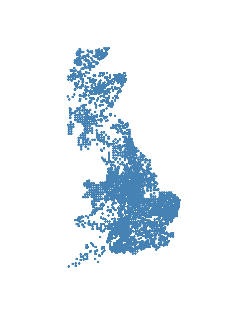
Now we can plot our spatial data:

> plot(voles, pch = 20, col = "steelblue")

1.3. Importing shapefiles

What if your data is already spatial? Then you probably have a shapefile. These files are made up of three mandatory files, with extensions .shp, .shx and .dbf, but other files that might be associated with a shapefile are .prj, .xml, .sbn, .sbx and .cpg. Sometimes the data you need is provided to you in this format already so it is useful to introduce here the functions that you need to read such data into R.

Now that we have a Spatial object in R, our voles SpatialPointsDataFrame, we can save it as a shapefile, so anytime we need it, all we need to do is read the file into R without having to go through the steps of setting the coordinates and defining the reference system. We can do so with the function writeOGR in the package rgdal. Install the package if you need to do so, then use this code to save your voles shapefile:

> library(rgdal)
> writeOGR(voles, dsn = "./data/voles.shp", layer = "voles", driver = "ESRI Shapefile")

The function writeOGR takes at least 3 arguments: the SpatialPointsDataFrame, SpatialLinesDataFrame, or a SpatialPolygonsDataFrame object that we want to save, the data source name (dsn) and the layer. The last two arguments can take different forms for different drivers, but for ESRI shapefile drivers the dsn is usually the name of the file with its .shp extension and layer is the name of the file without the extension. Take notice of the warning message, writeOGR has shortened your column names in the data.frame of attributes. This cannot be avoided with ESRI shapefile drivers but you can find a few suggestions for work around here. Now have a look at you data folder, how many files have you created?

We can now import the shapefile into R. We use the function readOGR, which takes similar arguments to writeOGR:

> voles <- readOGR(dsn = "./data/voles.shp", layer = "voles")
OGR data source with driver: ESRI Shapefile 
Source: "./data/voles.shp", layer: "voles"
with 46570 features
It has 42 fields

> summary(voles)
Object of class SpatialPointsDataFrame
Coordinates:
               min      max
coords.x1 -5.78827  1.77042
coords.x2 50.06594 58.65633
Is projected: FALSE 
proj4string : [+proj=longlat +ellps=WGS84 +no_defs]
Number of points: 46570
Data attributes:
...

2. Visualising Spatial Data

2.1. Plotting lines, points and polygons

We have already used the plot methods provided by sp, which builds on the traditional R plotting system. In this part of the tutorial we will plot other types of vector data (lines and polygons). We will use our voles dataset together with a few more spatial data for this part of the tutorial. In the data folder you will find two shapefiles:

coast
rivers_line Try read them in using the function readOGR as we did for the voles shapefile.

The SpatialLinesDataFrame has thousands small rivers that will make our points very difficult to see on the map, we can create a new object containing only the main rivers:

> main_rivers <- subset(rivers, LEGEND == "Main River, Middle" | LEGEND =="Main Rivers, Lower")

We can now plot these shapefiles on a single map.

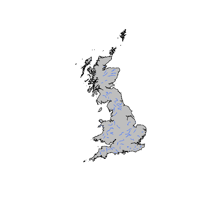
> plot(coast, col = "gray")
> lines(main_rivers, col = "royalblue1", lwd = 0.2)

Now plot the voles.

> points(voles, pch = 20, col = "orange")

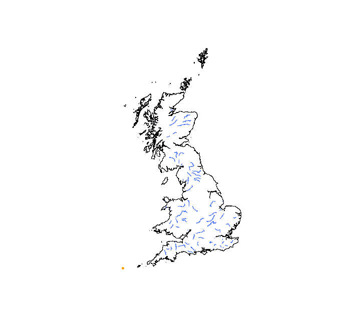
Where are our voles? This is a very common problem and one that took me hours to solve when I first started to deal with spatial data. What is happening here is actually quite simple. Remember the two conditions necessary for data to be spatial? Let’s have a look at the summary of our objects.

> summary(voles)
Object of class SpatialPointsDataFrame
Coordinates:
               min      max
coords.x1 -5.78827  1.77042
coords.x2 50.06594 58.65633
Is projected: FALSE 
proj4string : [+proj=longlat +ellps=WGS84 +no_defs]
Number of points: 46570
Data attributes:
...

> summary(main_rivers)
Object of class SpatialLinesDataFrame
Coordinates:
     min    max
x 144210 627730
y  75360 938680
Is projected: TRUE 
proj4string :
[+proj=tmerc +lat_0=49 +lon_0=-2 +k=0.9996012717 +x_0=400000 +y_0=-100000 +datum=OSGB36 +units=m +no_defs +ellps=airy
+towgs84=446.448,-125.157,542.060,0.1502,0.2470,0.8421,-20.4894]
Data attributes:
...

The first difference that you will notice is how different the Coordinates slot looks in the two objects, then you will notice the different proj4string. The coordinates reference systems for the two objects are different, therefore even if we know that they are on the same place on the Earth, they will not be mapped correctly when trying to plot them on the same map. We need to convert the reference system of some of our objects so that, in the end, they are all the same.

2.2. Projections and transformations

Looking at the Coordinates slot of the voles dataset we notice that the coordinates are in latitude and longitude degrees. This tells us that the data are unprojected. On the other hand, the data in the rivers and coast datasets are in meters, therefore projected. There exist many different projections and which one to use will depend on whch area on the globe you are mapping. In this case, working with the UK, the Transverse Mercator projection works well. The easiest thing to do to be able to visualise all our data on the same map is to project the voles dataset. We can use the function spTransform in the rgdal package.

> merc_proj <- proj4string(coast)
> voles_proj <- spTransform(voles, merc_proj)

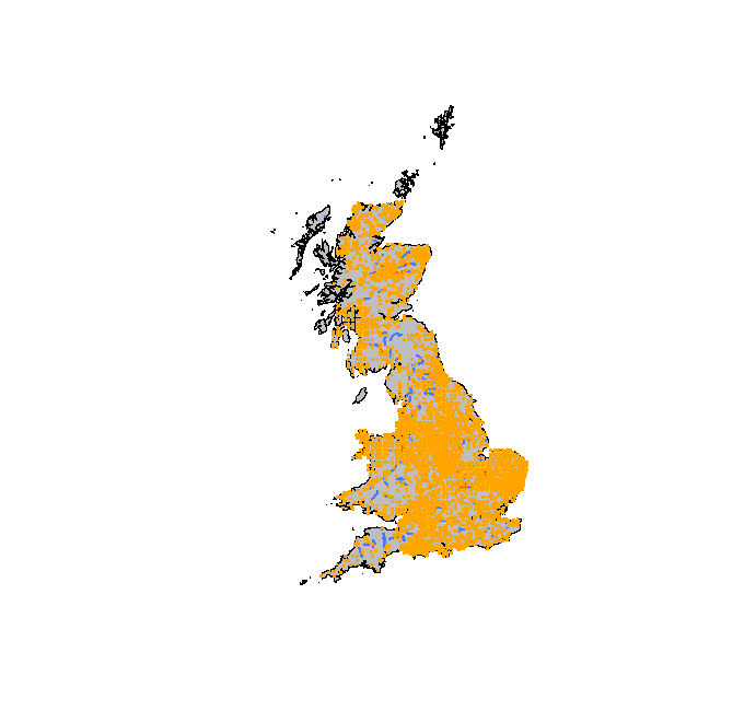
With the previous two lines we extracted the character string that describes the projection of the dataset coast with proj4string and we used spTransform to project our voles dataset. Do the same for the rivers dataset. Now we can try the plotting again.

> plot(coast, col="gray")
> lines(main_rivers, col = "royalblue1", lwd = 2)
> points(voles_proj, col = "orange", pch = ".", cex = 3)

Play around with the graphic parameters and make sure that you understand what they do.

3. Geoprocessing

Now that we know how to import our spatial data, visualise it and fix projection issues, we can start doing some manipulations.

The package rgeos has most of the geoprocessing functions that you would find in a GIS software, such as: union, distance, intersection, buffer, intersects, within and many more. We do not have the time to look at all of them, so we will concentrate on those operations that I found most common with biological spatial data, buffer, intersect and distance. Imagine you want to know if our voles’ occurrences are mainly in the vicinity of rivers. There are two ways we can answer this question. We can either create a buffer around our rivers and count how many points fall within this buffer compared to those outside or calculate the distance from every occurrence to the nearest river and count how many points are within a certain distance.

3.1. Buffer and Overlay

To create the buffer around our rivers we can use the function gBuffer in the package rgeos. If you don’t have this package you can install it using install.packages("rgeos").

> riv.buff <- gBuffer(rivers, width = 1)

> summary(riv.buff)
Object of class SpatialPolygons
Coordinates:
        min     max
x  8559.006  653839
y 13398.000 1216492
Is projected: TRUE 
proj4string :
[+proj=tmerc +lat_0=49 +lon_0=-2 +k=0.9996012717 +x_0=400000 +y_0=-100000 +datum=OSGB36 +units=m +no_defs +ellps=airy
+towgs84=446.448,-125.157,542.060,0.1502,0.2470,0.8421,-20.4894]

So we created a SpatialPolygons object which is a 1m buffer around the rivers. Notice that the CRS of our rivers object is already projected, so the coordinates are in meters. If the coordinates of rivers were in a geographic CRS then we would have had to project them before we could calculate a buffer. Now we can use the function gIntersect

> intersect <- gIntersects(voles_proj, riv.buff)
   Mode    TRUE    NA's 
logical       1       0

All of our voles’ occurrences are within 1m of rivers. Let’s replicate this result using a diferent approach.

3.2. Distance

We can select occurrences that are within a cetrain distance from the rivers by using the function gWithinDistance in the package rgeos.

> voles_sub <- gWithinDistance(voles_proj, rivers, dist = 1)
> summary(voles_sub)
   Mode    TRUE    NA's 
logical       1       0

Ok, that probably was not a very interesting question, we know that watervoles live close to waterways, but now you know how to make a buffer, intersect two different spatial objects and calculate distance between different spatial features. Also, you might have noticed that the distance operation took much less time to run compared to the intersect one. There usually is more than one way to do the same task in R, but some approaches will be more efficient than others, so it is worth experimenting to find the fastest option.

4. Rasters

This data model is widely used for storing data in regular rectangular cells, such as digital elevation models, satellite imagery and interpolated data from point measurements. Rasters are “gridded” data, which are stored as a grid of values, rendered on a map as pixels. Each pixel value represents an area on the Eart’s surface. Different types of data can be stored in this format, including continuous data (heigth, depth etc.) and categorical data (land use categories). Raster data also come in different formats. Today we will work with GeoTiff format, which is a standard .tif image format with additional spatial information embedded in the file as tags.

We will use the package raster to import the raster data and do some manipulations, so install the package with install.packages("raster") and load it with library(raster).

4.1. Import rasters and change projection

To download the file you need for this part of the tutorial, go to this link. Once you’ve downloaded the file save it in the same data folder where you have all the other files. Now in your data folder there is a .tif file, a GeoTiff raster with information about land cover in the UK. We can use the function raster to import this file and then use plot to visualise it.

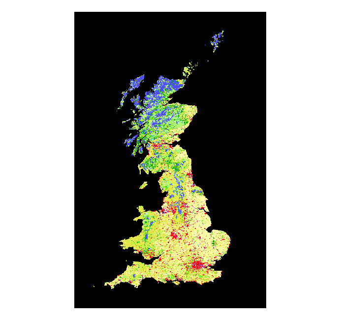
> land_use <- raster("./data/Land_Use.tif")
> plot(land_use)

Let’s familiarise ourselves with this object.

> land_use
class       : RasterLayer 
dimensions  : 13068, 8465, 110620620  (nrow, ncol, ncell)
resolution  : 99.99333, 99.99333  (x, y)
extent      : 3076305, 3922748, 3010302, 4317015  (xmin, xmax, ymin, ymax)
coord. ref. : +proj=laea +lat_0=52 +lon_0=10 +x_0=4321000 +y_0=3210000 +ellps=GRS80 +towgs84=0,0,0,0,0,0,0 +units=m +no_defs 
data source : H:\StudyGroup\SG-T7-SpatialR\data\Land_Use.tif 
names       : Land_Use 
values      : 1, 44  (min, max)

The first line tells us that we are dealing with an object of class RasterLayer. The second line gives us the dimensions of the raster, but number of cells is not a very informative measure without the information stored in the next 2 lines, the resolution and the extent. The latter tells us which region our data covers and the first gives a measure of how detailed the data is. The slot coord. ref. tells us the coordinate reference system of our raster. We can see that it is projected (+units=m), but it is in a different projection compared to the rest of our data. Before we can do any manipulation on these data we need to reproject the raster. This works the same as for vector data, but uses a different function: projectRaster. This is going to take a while because it is a big file!

> land_use_proj <- projectRaster(land_use, crs = merc_proj)

Let’s plot our voles occurrences on top of the land use raster.

> plot(land_use_proj)
> points(voles_proj, col = "black", pch = ".", cex = 3)

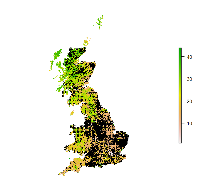
Looks like we have lost the categorical nature of the raster data AND it took forever! It might be better to reproject the vector data in this case.

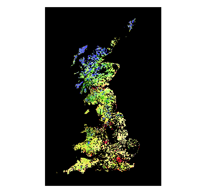
> voles_proj2 <- spTransform(voles, proj4string(land_use))

Plot again.

> plot(land_use)
> points(voles_proj2, col = "black", pch = ".", cex = 3)

4.2. Some geoprocessing

Imagine we want to know in which land cover class water voles are more likely to be. The simplest way of doing this is by finding out what land use category is under each water vole occurrence. This operation is a point-raster overlay, or an extraction.

> land_voles <- extract(land_use, voles_proj2)
> str(land_voles)

The function extract returns a vector of the same length as our point dataframe containing the values of the raster at the points’ locations. Now we can use the clc_legend.csv file to obtain the lables for the land use classes indentified by these numbers. The following code loads the file, creates a new column in the voles dataframe to store the associated value of land use and then associates a label from the legend to each of these values.

> legend <- read.csv("./data/Legend/clc_legend.csv", row.names = "GRID_CODE", sep = ";")
> voles_proj2$LandUse <- land_voles
> voles_proj2$landUseCode3 <- legend[as.character(land_voles), "LABEL3"]

Now we can produce a table that will tell us how many occurrences of voles were recorded per land use class.

> table(voles_proj2$landUseCode3)

Which land use class has the most occurrences?

> which(table(voles_proj2$landUseCode3) == max(table(voles_proj2$landUseCode3)))
Non-irrigated arable land 
                       28

5. Summary and useful links

This tutorial is only a basic introduction to mapping and geoprocessing in R. The idea was to introduce the types of object that you will be dealing with in spatial analysis so they are not that obscure and scary anymore. Today you have learnt how to transform a data.frame into a Spatial object, import shapefiles and GeoTiff files, make basic maps and conduct some simple geoprocessing operations. This is a huge topic and, as always, the R community is highly productive ao that the number of packages for geospatial data is increasing very fast. Have a look at this list of R packages on analysis of spatial data put together by Roger Bivand. I have put together a list of resources that you might find useful if you want to know more about geospatial data in R:

Barry Rowlingson’s excellent online tutorial Geospatial Data in R and Beyond
neon’s series Introduction to working with raster data in R
Roger Bivand’s fabulous book Applied Spatial Data Analysis with R
Francisco Rodriguez-Sanchez’s great tutorial on Spatial data in R: Using R as a GIS

Open Spatial Analysis 1 - Handling spatial data in R

1. Classes for Spatial Data in R and how to import the data

1.1. The Spatial class and its subclasses

1.2. Importing your data and making it spatial

1.3. Importing shapefiles

2. Visualising Spatial Data

2.1. Plotting lines, points and polygons

2.2. Projections and transformations

3. Geoprocessing

3.1. Buffer and Overlay

3.2. Distance

4. Rasters

4.1. Import rasters and change projection

4.2. Some geoprocessing

5. Summary and useful links

1.1. The `Spatial` class and its subclasses